Intersection over Union (IoU)#
Intersection over Union (IoU) measures the ratio of the intersection and the union between ground truth and inference, ranging from 0 to 1 where 1 indicates a perfect match. The objective of this metric is to compare inferences to ground truths by measuring similarity between them.
As the name suggests, the IoU of two instances (\(\text{A}\) and \(\text{B}\)) is defined as:
-
API Reference:
iou↗
When Do I Use IoU?#
It is often used to compare two geometries (e.g., BoundingBox,
Polygon or SegmentationMask)
in object detection, instance segmentation, or semantic segmentation workflows. In multi-label classification, IoU,
more likely known as the Jaccard index, is used to compare set of
inference labels for a sample to the corresponding set of ground truth labels. Moreover, there are workflows such as
action detection and
video moment retrieval where IoU measures the temporal overlap
between two time-series snippets.
Because IoU can be used on various types of data, let's look at how the metric is defined for some of these data types:
2D Axis-Aligned Bounding Box#
Let's consider two 2D axis-aligned bounding boxes, \(\text{A}\) and \(\text{B}\), with the origin of the coordinates being the top-left corner of the image, and to the right and down are the positive directions of the \(x\) and \(y\) axes, respectively. This is the most common coordinate system in computer vision.


Guides: Commonly Used Bounding Box Representations
A bounding box is often defined by the \(x\) and \(y\) coordinates of the top-left and bottom-right corners. This is
the format used in this guide and in the kolena package.
Another commonly used representation is the \(x\) and \(y\) coordinates of bounding box center, along with the width and height of the box.
In order to compute IoU for two 2D bounding boxes, the first step is identifying the area of the intersection box, \((\text{A} \cap \text{B})\). This is the highlighted overlap region in the image above. The two coordinates of the intersection box, top-left and bottom-right corners, can be defined as:
Once the intersection box \((\text{A} \cap \text{B})\) is identified, the area of the union, \((\text{A} \cup \text{B})\), is simply a sum of the area of \(\text{A}\) and \({\text{B}}\) minus the area of the intersection box.
Finally, IoU is calculated by taking the ratio of the area of intersection box and the area of the union region.
Examples: IoU of 2D Bounding Boxes#
The following examples show what IoU values look like in different scenarios with 2D bounding boxes:
Example 1: overlapping bounding boxes


Example 2: non-overlapping bounding boxes


Example 3: completely matching bounding boxes


Segmentation Mask#
A segmentation mask is a 2D image where each pixel is a class label commonly used in semantic segmentation workflow. The inference shape matches the ground truth shape (width and height), with a channel depth equivalent to the number of class labels to be predicted. Each channel is a binary mask that labels areas where a specific class is present:
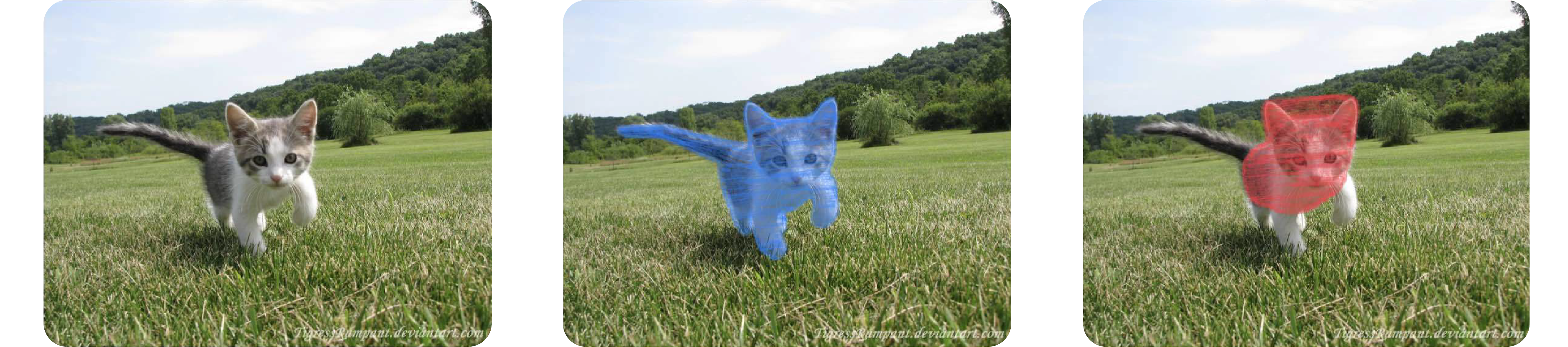
The IoU metric measures the intersection (the number of pixels common between the ground truth and inference masks, true positive (TP)) divided by the union (the total number of pixels present across both masks, TP + false negative (FN) + false positive (FP)). And here is the formula for the IoU metric for a segmentation mask:
Let’s look at what TP, FP, and FN look like on a segmentation mask:
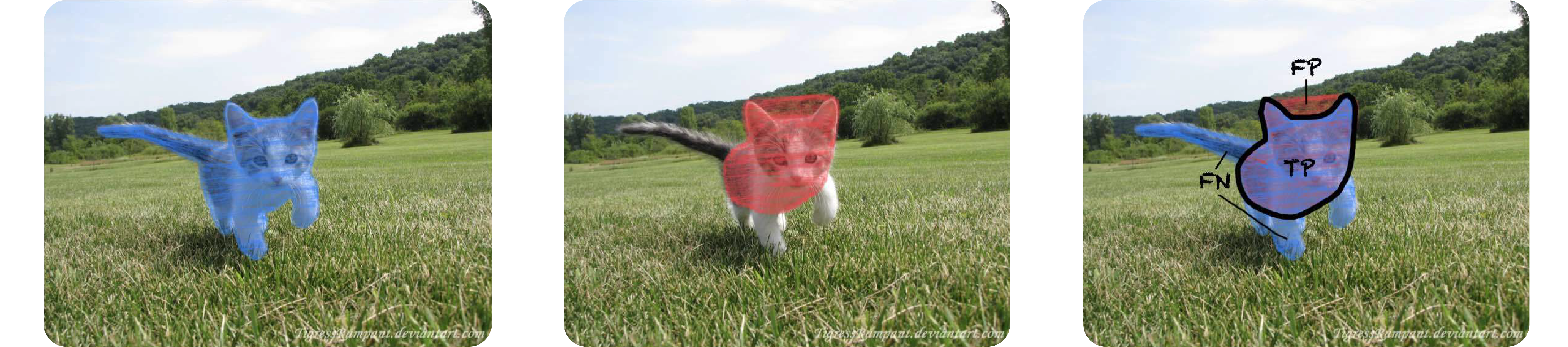
From the cat image shown above, when you overlay the ground truth and inference masks, the pixels that belong to both masks are TP. The pixels that only exist in the ground truth mask are FNs, and the pixels that only exist in the inference mask are FPs. Let's consider the following pixel counts for each category:
| # True Positives | # False Positives | # False Negatives |
|---|---|---|
| 100 | 25 | 75 |
Then the IoU becomes:
Set of Labels#
The set of labels used in multi-label classification workflow is often a
binarized list with a
number of label elements, for example, let’s say there are three classes, Airplane, Boat, and Car, and a sample
is labeled as Boat and Car. The binary set of labels would then be \([0, 1, 1]\), where each element represents each
class, respectively.
Similar to the segmentation mask, the IoU or Jaccard index metric for the ground truth/inference labels would be the size of the intersection of the two sets (the number of labels common between two sets, or TP) divided by the size of the union of the two sets (the total number of labels present in both sets, TP + FN + FP):
The IoU for multi-label classification is defined per class. This technique, also known as one-vs-the-rest (OvR), evaluates each class as a binary classification problem. Per-class IoU values can then be aggregated using different averaging methods. The popular choice for this workflow is macro, so let’s take a look at examples of different averaged IoU/Jaccard index metrics for multiclass multi-label classification:
Example: Macro IoU of Multi-label Classification#
Consider the case of multi-label classification with classes Airplane, Boat, Car:
| Set | Sample #1 | Sample #2 | Sample #3 | Sample #4 |
|---|---|---|---|---|
| ground truth | Airplane, Boat, Car |
Airplane, Car |
Boat, Car |
Airplane, Boat, Car |
| inference | Boat |
Airplane, Boat, Car |
Airplane, Boat, Car |
Airplane, Boat, Car |
Limitations and Biases#
IoU works well to measure the overlap between two sets, whether they are types of geometry or a list of labels. However,
this metric cannot be directly used to measure the overlap of an inference and iscrowd ground truth, which is an
annotation from COCO Detection Challenge Evaluation used to label a large
groups of objects (e.g., a crowd of people). Therefore, the inference is expected to take up a small portion of the
ground truth region, resulting in a low IoU score and a pair not being a valid match. In this scenario, a variation of
IoU, called Intersection over Foreground (IoF), is preferred.
This variation is used when there are ground truth regions you want to ignore in evaluation, such as iscrowd.
The second limitation of IoU is measuring the localization performance of non-overlaps. IoU ranges from 0 (no overlap) to 1 (complete overlap), so when two bounding boxes have zero overlap, it’s hard to tell how bad the localization performance is solely based on IoU. There are variations of IoU, such as signed IoU (SIoU) and generalized IoU (GIoU), that aim to measure the localization error even when there is no overlap. These metrics can replace IoU metric if the objective is to measure the localization performance of non-overlaps.