ROC Curve#
A receiver operating characteristic (ROC) curve is a plot that is used to evaluate the performance of binary classification models by using the true positive rate (TPR) and the false positive rate (FPR). The curve is built with the TPR on the y-axis and the FPR on the x-axis computed across many thresholds, showing a trade-off of how TPR and FPR values change when a classification threshold changes.
Guides: TPR and FPR
The TPR is also known as sensitivity or recall, and it represents the proportion of true positive inferences (correctly predicted positive instances) among all actual positive instances. The FPR is the proportion of false positive inferences (incorrectly predicted positive instances) among all actual negative instances. Read the true positive rate (TPR) and the false positive rate (FPR) guides to learn more about these metrics.
-
API Reference:
CurvePlot↗
Implementation Details#
The curve’s points (TPRs and FPRs) are calculated with a varying threshold, and made into points (TPR values on the y-axis and FPR values on the x-axis). TPR and FPR metrics are threshold-dependent where a threshold value must be defined to compute them, and by computing and plotting these two metrics across many thresholds we can check how these metrics change depending on the threshold.
Thresholds Selection
Threshold ranges are very customizable. Typically, a uniformly spaced range of values from 0 to 1 can model a ROC curve, where users pick the number of thresholds to include. Another common approach to picking thresholds is collecting and sorting the unique confidences of every prediction.
Example: Binary Classification#
Let's consider a simple binary classification example and plot a ROC curve at a uniformly spaced range of thresholds. The table below shows eight samples (four positive and four negative) sorted by their confidence score. Each inference is evaluated at each threshold: 0.25, 0.5, and 0.75. It's a negative prediction if its confidence score is below the evaluating threshold; otherwise, it's positive.
| Sample | Inference @ 0.25 | Inference @ 0.5 | Inference @ 0.75 | |
|---|---|---|---|---|
| Positive | 0.9 | Positive | Positive | Positive |
| Positive | 0.8 | Positive | Positive | Positive |
| Negative | 0.75 | Positive | Positive | Positive |
| Positive | 0.7 | Positive | Positive | Negative |
| Negative | 0.5 | Positive | Positive | Negative |
| Positive | 0.35 | Positive | Negative | Negative |
| Negative | 0.3 | Positive | Negative | Negative |
| Negative | 0.2 | Negative | Negative | Negative |
As the threshold increases, there are fewer true positives and fewer false positives, most likely yielding lower TPR and FPR. Conversely, decreasing the threshold may increase both TPR and FPR. Let's compute the TPR and FPR values at each threhold using the following formulas:
| Threshold | TP | FP | FN | TN | TPR | FPR |
|---|---|---|---|---|---|---|
| 0.25 | 4 | 3 | 0 | 1 | \(\frac{4}{4}\) | \(\frac{3}{4}\) |
| 0.5 | 3 | 2 | 1 | 2 | \(\frac{3}{4}\) | \(\frac{2}{4}\) |
| 0.75 | 2 | 1 | 2 | 3 | \(\frac{2}{4}\) | \(\frac{1}{4}\) |
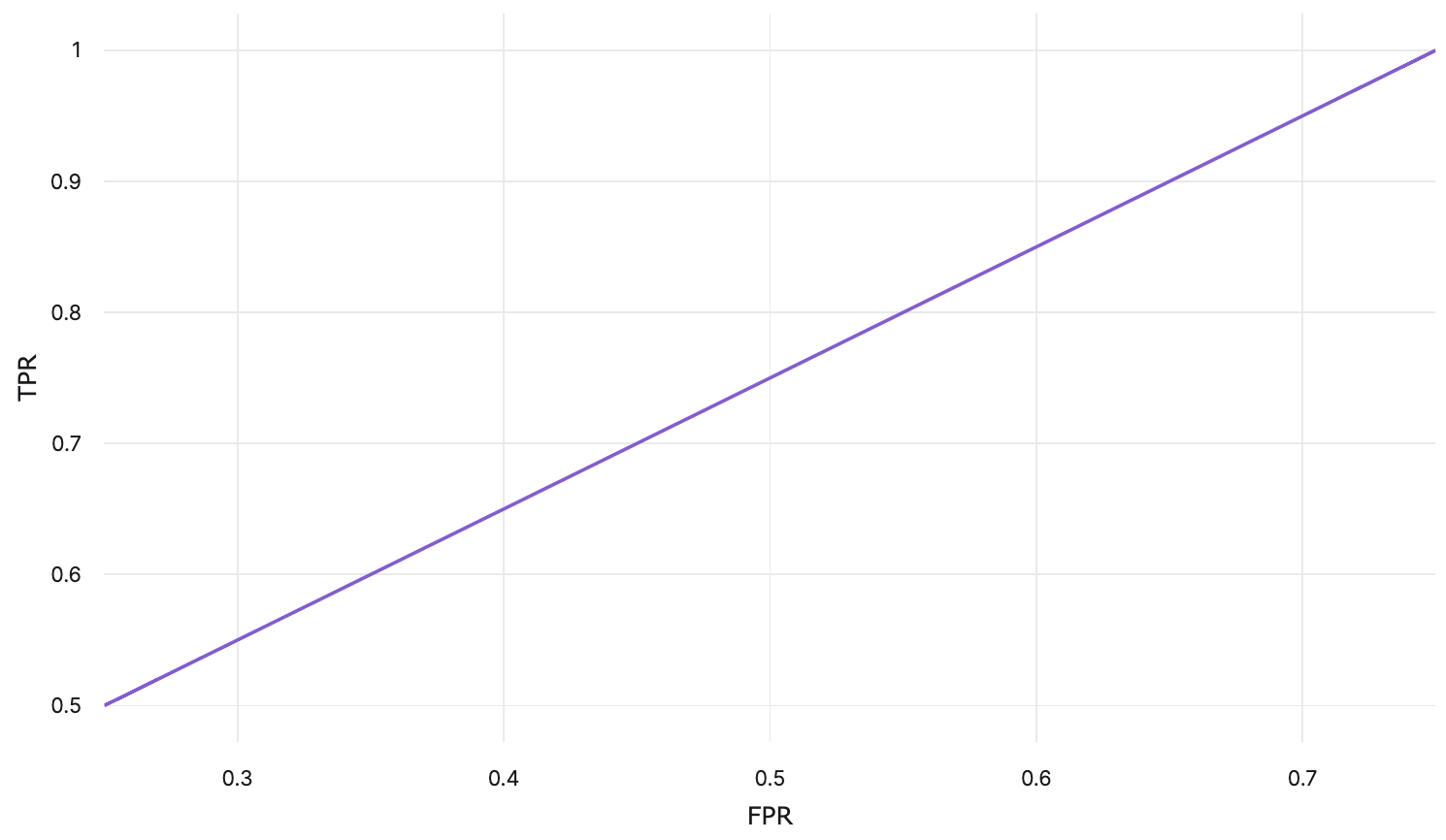
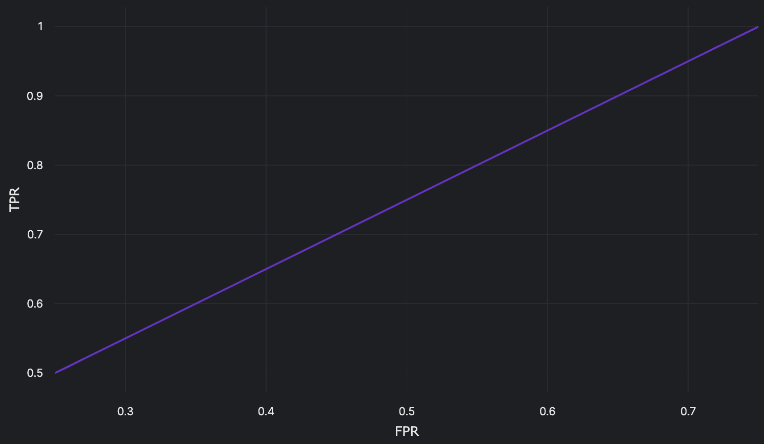
Using these TPR and FPR values, a ROC curve can be plotted:
Example: Multiclass Classification#
For multiple classes, a curve is plotted per class by treating each class as a binary classification problem. This
technique is known as one-vs-rest (OvR). With this strategy, we can have n ROC
curves for n unique classes.
Let's take a look at a multiclass classification example and plot per class ROC curves for the same three
thresholds that we used in the example above: 0.25, 0.5, and 0.75. In this example, we have three classes:
Airplane, Boat, and Car. The multiclass classifier outputs a confidence score for each class:
| Sample # | Label | Airplane Confidence |
Boat Confidence |
Car Confidence |
|---|---|---|---|---|
| 1 | Airplane |
0.9 | 0.05 | 0.05 |
| 2 | Airplane |
0.7 | 0.05 | 0.25 |
| 3 | Airplane |
0.25 | 0.25 | 0.5 |
| 4 | Boat |
0.6 | 0.25 | 0.15 |
| 5 | Boat |
0.4 | 0.5 | 0.1 |
| 6 | Car |
0.25 | 0.25 | 0.5 |
| 7 | Car |
0.05 | 0.7 | 0.25 |
Just like the binary classification example, we are going to determine whether each inference is positive or negative
depending on the evaluating threshold, so for class Airplane:
| Sample # | Sample | Airplane Confidence ↓ |
Inference @ 0.25 | Inference @ 0.5 | Inference @ 0.75 |
|---|---|---|---|---|---|
| 1 | Positive | 0.9 | Positive | Positive | Positive |
| 2 | Positive | 0.7 | Positive | Positive | Negative |
| 4 | Negative | 0.6 | Positive | Positive | Negative |
| 5 | Negative | 0.4 | Positive | Negative | Negative |
| 3 | Positive | 0.25 | Positive | Negative | Negative |
| 6 | Negative | 0.25 | Positive | Negative | Negative |
| 7 | Negative | 0.05 | Negative | Negative | Negative |
And the TPR and FPR values for class Airplane can be computed:
| Threshold | TP | FP | FN | TN | Airplane TPR |
Airplane FPR |
|---|---|---|---|---|---|---|
| 0.25 | 3 | 3 | 0 | 1 | \(\frac{3}{3}\) | \(\frac{3}{4}\) |
| 0.5 | 2 | 1 | 1 | 3 | \(\frac{2}{3}\) | \(\frac{1}{4}\) |
| 0.75 | 1 | 0 | 2 | 4 | \(\frac{1}{3}\) | \(\frac{0}{4}\) |
We are going to repeat this step to compute TPR and FPR for class Boat and Car.
| Threshold | Airplane TPR |
Airplane FPR |
Boat TPR |
Boat FPR |
Car TPR |
Car FPR |
|---|---|---|---|---|---|---|
| 0.25 | \(\frac{3}{3}\) | \(\frac{3}{4}\) | \(\frac{2}{2}\) | \(\frac{3}{5}\) | \(\frac{2}{2}\) | \(\frac{2}{5}\) |
| 0.5 | \(\frac{2}{3}\) | \(\frac{1}{4}\) | \(\frac{1}{2}\) | \(\frac{1}{5}\) | \(\frac{1}{2}\) | \(\frac{1}{5}\) |
| 0.75 | \(\frac{1}{3}\) | \(\frac{0}{4}\) | \(\frac{0}{2}\) | \(\frac{0}{5}\) | \(\frac{0}{2}\) | \(\frac{0}{5}\) |
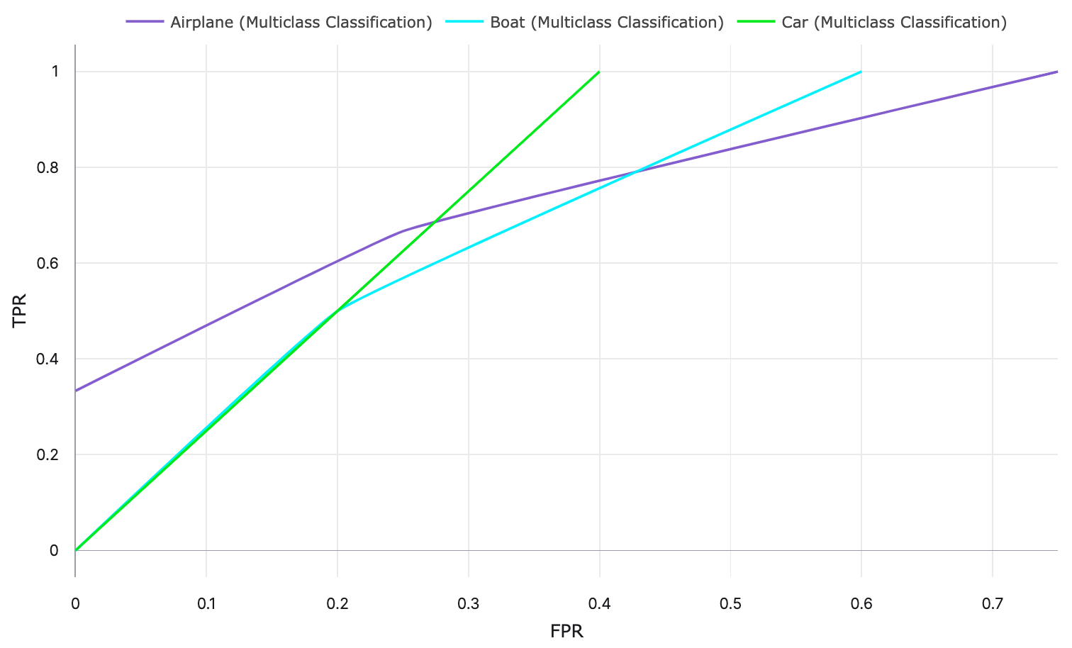
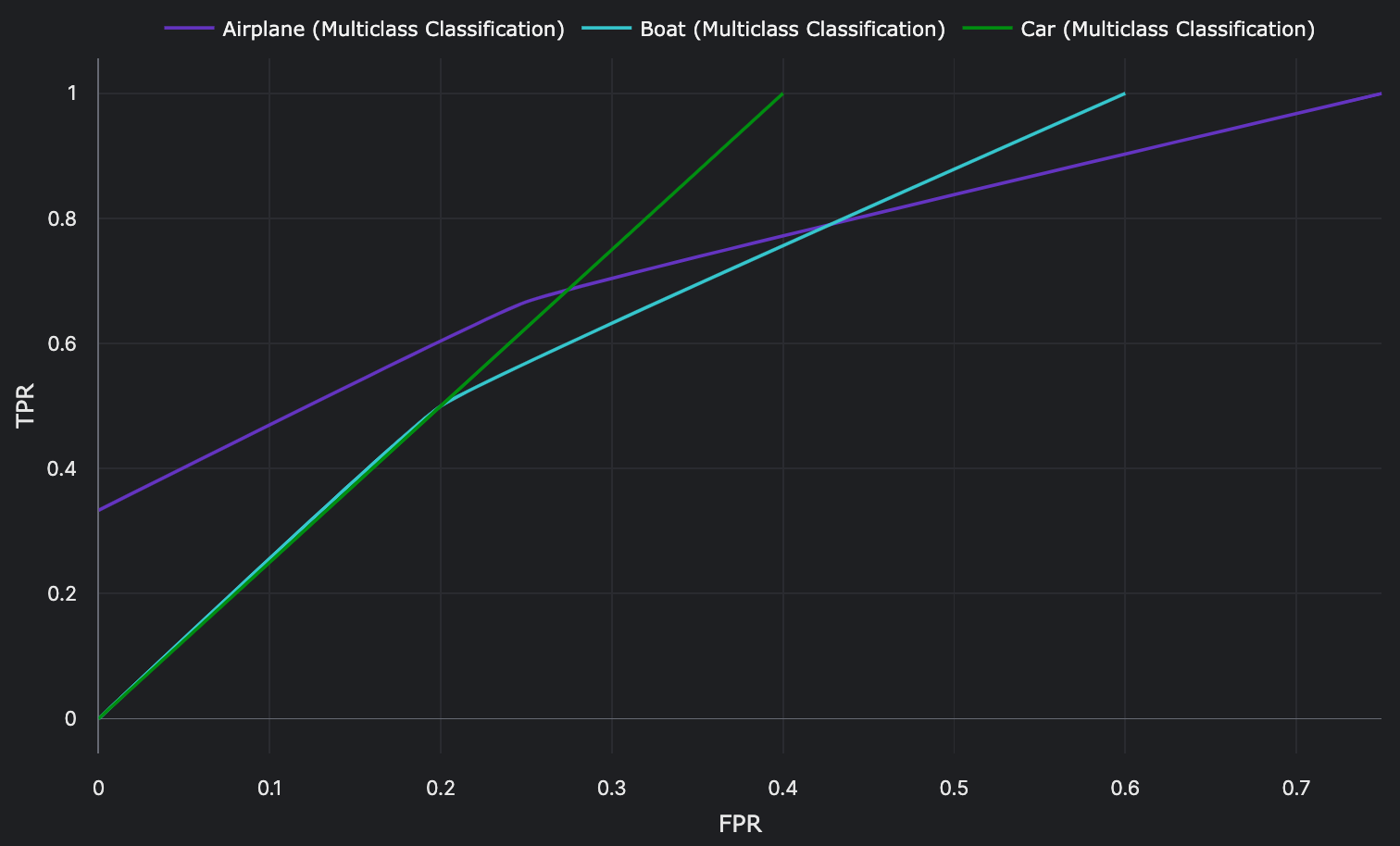
Using these TPR and FPR values, per class ROC curves can be plotted:
Area Under the ROC Curve (AUC ROC)#
The area under the ROC curve (AUC ROC) is a threshold-independent metric that summarizes the performance of a model depicted by a ROC curve. A perfect classifier would have an AUC ROC value of 1. The greater the area, the better a model performs at classifying the positive and negative instances. Using AUC ROC metric alongside other evaluation metrics, we can assess and compare the performance of different models and choose the one that best suits their specific problem.
Let's take a look at the binary classification example again. Given the following TPR and FPR values, the AUC ROC can be computed:
| Threshold | TP | FP | FN | TN | TPR | FPR |
|---|---|---|---|---|---|---|
| 0.25 | 4 | 3 | 0 | 1 | \(\frac{4}{4}\) | \(\frac{3}{4}\) |
| 0.5 | 3 | 2 | 1 | 2 | \(\frac{3}{4}\) | \(\frac{2}{4}\) |
| 0.75 | 2 | 1 | 2 | 3 | \(\frac{2}{4}\) | \(\frac{1}{4}\) |
The area under the curve can computed by taking an integral along the x-axis using the composite trapezoidal rule:
For Python implementation, we recommend using NumPy's
np.trapz(y, x) or
scikit-learn's sklearn.metrics.auc.
Limitations and Biases#
While ROC curves and AUC ROC are widely used in machine learning for evaluating classification models, they do have limitations and potential biases that should be considered:
- Sensitive to Class Imbalance: Classes with too few data points may have ROC curves that are poor representations of actual performance or overall performance. The performance of minority classes may be less accurate compared to a majority class.
- Partial Insight to Model Performance: ROC curves only gauge TPR and FPR based on classifications, they do not surface misclassification patterns or reasons for different types of errors. AUC ROC treats false positives and false negatives equally which may not be appropriate in situations where one type of error is more costly or impactful than the other. In such cases, other evaluation metrics like precision or PR curve can be used.
- Dependence on Threshold: The values of the thresholds affect the shape of ROC curves, which can affect how they are interpreted. Having a different number of thresholds, or having different threshold values, make ROC curve comparisons difficult.